Matplotlib charts

Matplotlib is a powerful graph and chart rendering library. Learn how to master it to make amazing illustrations of your data. Install the library matplotlib to proceed.

The following code all uses the import statement of:

import matplotlib.pyplot as plt

Histogram

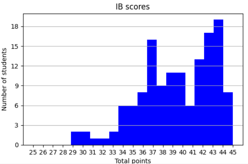
data = [29,29,30,...] # Extract of data
plt.rcParams["figure.figsize"] = (10,10)
plt.xlabel('Total points')
plt.ylabel('Number of students')
plt.yticks([0,3,6,9,12,15,18,21])
plt.grid(True, axis='y')
plt.title('IB scores')
plt.hist(data, range=(20,45), bins=26, color='blue')
plt.show()

Bar chart

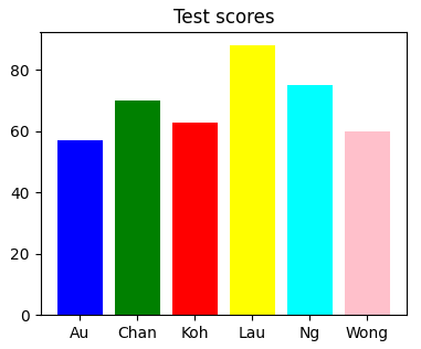
names = ['Au','Chan','Koh','Lau','Ng','Wong']
scores = [57, 70, 63, 88, 75, 60]
color_list = ['blue','green','red','yellow','cyan','pink']
plt.title('Test scores')
plt.bar(names, scores, color=color_list)   # plt.barh() will give a horizontal chart
plt.show()

Plot chart

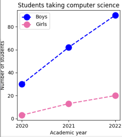
Incidentally, the following two charts are based on real data that illustrate how Computer Science still has a long way to go in order to reach equity and parity!

years = [2020, 2021, 2022]
boys = [30,62,90]
girls = [3,13,20]
plt.xlabel('Academic year')
plt.xticks(years)
plt.ylabel('Number of students')
plt.title('Students taking computer science')
plt.plot(years, boys, label="Boys", color='blue', marker='o', \
   linestyle='dashed', linewidth=2, markersize=12)
plt.plot(years, girls, label="Girls", color='#e96daa', marker='o', \
   linestyle='dashed', linewidth=2, markersize=12)
plt.legend()
plt.show()

Pie chart

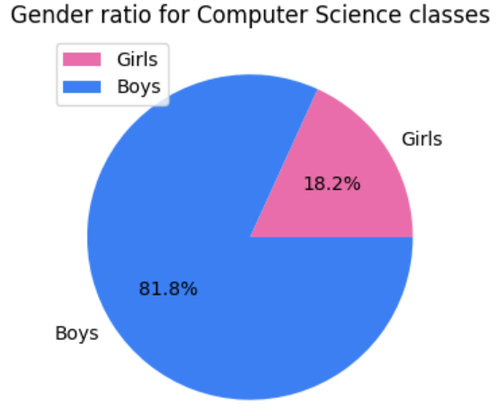
names = ["Girls","Boys"]
values = [20,90]
colors = ["#e96daa", "#3b7ff2"]
plt.title('Gender ratio for Computer Science classes')
plt.pie(values, labels=names, colors=colors, autopct='%1.1f%%')
plt.legend()
plt.show()

Scatter diagram

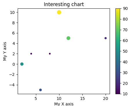
# SCATTER DIAGRAM 
# With size/colour variation 
x = [ 2, 4, 6, 8,10,12,20]
y = [ 0, 2,-5, 2,10, 5, 5]
s = [50,10,30,10,90,70,20]
plt.xlabel('My X axis')
plt.ylabel('My Y axis')
plt.title('Interesting chart')
plt.scatter(x, y, s=s, c=s) # s=sizes, c=colors
plt.colorbar()
plt.show()

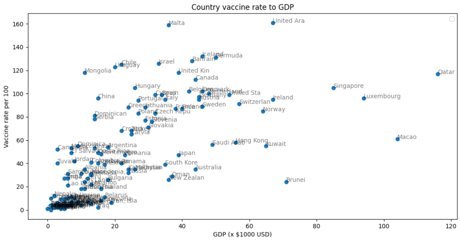
# SCATTER DIAGRAM
# Data sourced from ourworldindata.org as of 13/7/2021
labels = ["Australia", .... ] # list of country names
y = [35, ...] # vaccine doses per 100
x = [44, ...] # GDP in 1000s of USD
plt.rcParams["figure.figsize"] = (10,10) # (inches)
plt.xlabel('GDP (x $1000 USD)')
plt.ylabel('Vaccine rate per 100')
plt.title('Country vaccine rate to GDP')
plt.scatter(x,y) # Create chart
for i in range(len(labels)): # label each coordinate
    plt.annotate(labels[i], (x[i], y[i]), alpha=0.5)
plt.show()

Box and violin plots

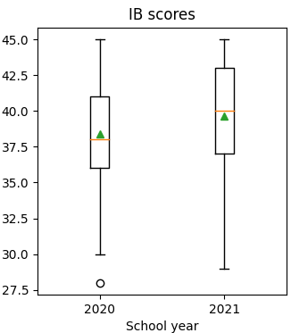
# BOX PLOTS
data2020 = [28,30,30,...] # Extract
data2021 = [29,29,30,...] # Extract
data = [data2020, data2021]
plt.title('IB scores')
plt.xlabel('School year')
ax = plt.gca()
ax.axes.xaxis.set_ticklabels([2020,2021])
plt.boxplot(data, showmeans=True)
plt.show()

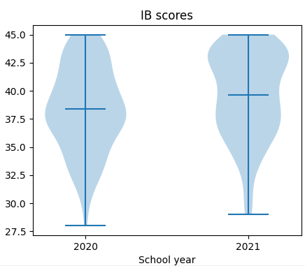
# VIOLIN PLOTS
data2020 = [28,30,30,...] # Extract
data2021 = [29,29,30,...] # Extract
data = [data2020, data2021]
plt.title('IB scores')
plt.xlabel('School year')
ax = plt.gca()
ax.set_xticks([1,2])
ax.set_xticklabels([2020,2021])
plt.violinplot(data, showmeans=True)
plt.show()

Saving charts

All the above examples use plt.show() to render the chart on screen. You can also have Python save the chart as an image using the plt.savefig() function as follows:

plt.savefig("file.png", format: "png")